How can a country build its own 1000 Genomes Project?

Recent national genome initiatives highlight the growing need for population-specific genomic resources. After reading VN1K: a genome graph-based and function-driven multi-omics and phenomics resource for the Vietnamese population and EGP1K: Whole-Genome Sequencing of 1,024 Egyptians Characterizes Population Structure and Genetic Diversity, it becomes clear that building a national-scale 1000-genome project is increasingly important for understanding genetic diversity, improving disease research, and enabling precision medicine.
In this blog, I outline how a country can design and implement a project at a similar scale — from sample collection to cohort-level genomic analysis. This discussion focuses on the technical and architectural aspects of building the 1000-genome resource. It does not cover the downstream data platform or user portal for accessing processed data, which will be explored in a separate article.
The goal is to provide a practical, scalable roadmap that countries — especially those with emerging genomics infrastructure — can adapt to their own national genome initiatives.
1. The Vision — Why Countries Need Their Own 1000 Genomes Project
The original 1000 Genomes Project (2008-2015) was a watershed moment in human genomics—it created the first comprehensive catalog of global genetic variation, providing a reference map that democratized variant calling and population genetics. But here's the catch: that data, while invaluable globally, doesn't fully represent your country's population, healthcare challenges, or genetic landscape.
1.1. The Global Reference Isn't Enough
Modern genome analysis relies heavily on population-specific variant frequencies. When you're doing variant interpretation, rare disease diagnosis, or pharmacogenomics, you need to know: How common is this variant in the population I'm treating? The 1000 Genomes Project surveyed ~2,500 individuals across diverse populations, but the genetic variation in your local population—shaped by unique migration histories, founder effects, and evolutionary pressures—may differ significantly.
Clinical implications are real:
- A variant marked as "rare" globally might be common in your population
- Disease association studies require local allele frequency data
- Precision medicine strategies must account for population-specific risk alleles
- Rare disease diagnosis becomes more accurate with local context
1.2. Sovereignty and Data Ownership
Large-scale genomic projects generate not just data—they generate infrastructure, expertise, and economic value. Countries that build their own projects gain:
- Data sovereignty: Complete control over sensitive health data rather than relying on international consortiums
- Research leadership: Ability to conduct population-specific studies without external dependencies
- Economic opportunity: Local biotech ecosystems can leverage the data for drug discovery and diagnostics
- Healthcare innovation: Direct pathway from research insights to clinical practice
1.3. Learning from Existing National Programs Led By Government
The good news: many countries have already built or are building large-scale genome projects. Here's what they've taught us:
- UK Biobank sequenced 500k+ genomes linked to longitudinal health records, demonstrating how genomic data at scale enables population-wide disease discovery and precision medicine
- All of Us Research Program (US) demonstrates how to scale to 1 million+ genomes with robust data governance and participant engagement
- Biobank Japan shows how to integrate genomic data with longitudinal health records for disease association studies
- Singapore's National Precision Medicine Program illustrates how population-specific allele frequencies improve diagnosis and treatment in resource-constrained settings
- China's BGI and national initiatives showcase infrastructure for processing massive cohorts at scale
- Australia's Australian Genomics demonstrates federated governance across multiple institutions and states
- Others many more genomics population biobank is establishing with efforts to support for their own contries: South Korea, Sweden, Finland, etc
These programs share common patterns: they all standardized variant calling, implemented joint genotyping strategies, built cohort-wide analytics layers, and invested heavily in data governance. The technical blueprint is proven—now it's about adapting it to your country's resources, population, and healthcare priorities.
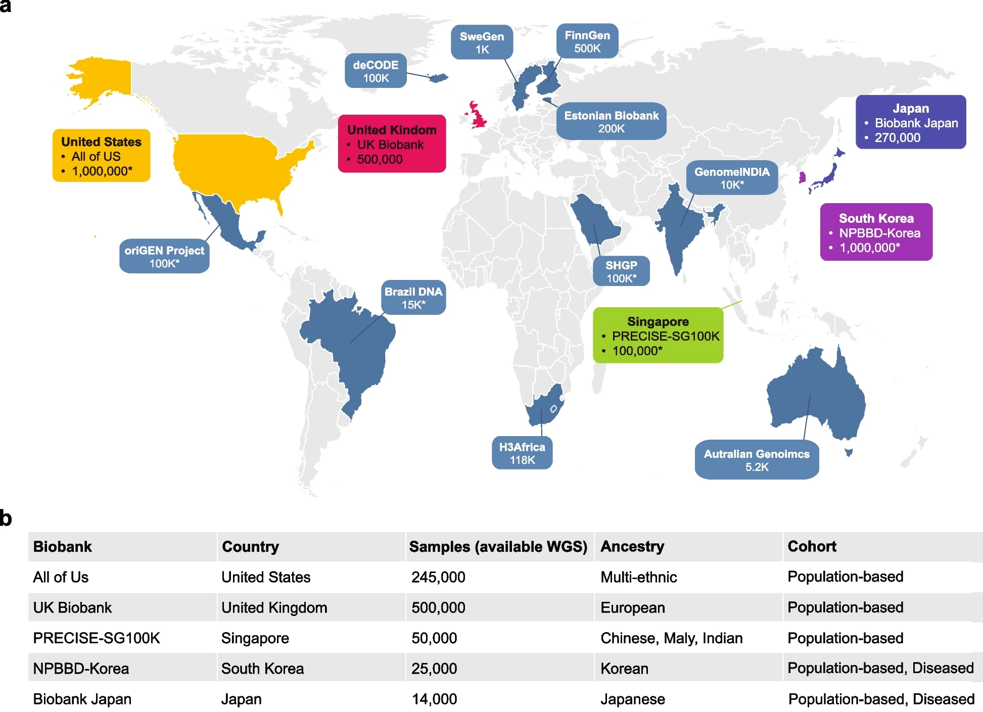 Figure 1: Overview of genomic resources in the national biobanks. a Geographical distribution of the biobanks, with the sample numbers representing the total cohort size targeted or achieved by each biobank. Major biobanks possessing large-scale WGS datasets exceeding 10,000 individuals are highlighted. An asterisk (“*”) indicates the targeted cohort size. b Detailed information on WGS sample sizes, ancestry composition, and health conditions of the respective biobank datasets were recently disclosed
Reference: https://link.springer.com/article/10.1186/s44342-025-00040-9
1.4. Learning from Existing Programs Led By Private Companies
While national and government-funded programs dominate the landscape, private companies and organizations have also built impressive large-scale genomic initiatives. Understanding their approach offers valuable lessons on infrastructure, scaling, and data governance.
Direct-to-Consumer (DTC) Companies
- 23andMe - 15M+ genotyped users with proprietary research database and health insights. Demonstrates consumer engagement at massive scale, though with privacy considerations
- AncestryDNA - 20M+ genotyped users focused on ancestry and family connections. Shows how genealogical context drives adoption and participation
Pharmaceutical & Drug Development
- Regeneron Genetics Center (DiscovEHR) - Exomes of ~50k patients linked to electronic health records. Gold standard for pharma-healthcare collaboration; proves that clinical data integration dramatically increases research value
- Genentech/Roche - Built internal genomic databases from clinical trials and partner networks. Focus on precision oncology and rare diseases
- GSK (GlaxoSmithKline) - Genomics partnerships acquiring genetic databases for target identification. Demonstrates how pharma funds large-scale infrastructure
Clinical Genomics & Diagnostic Companies
- Invitae - ~5M genetic testing records (largest clinical genetics lab). Standardized variant calling across millions of diagnostic samples shows how clinical labs maintain quality at scale
- Tempus - 10M+ de-identified genomic records with AI-powered analysis. Cancer-focused platform demonstrates the value of unified analytics layers
- Foundation Medicine (Roche) - 1.5M+ patient profiles. Precision oncology at scale—proves that focused cohorts can drive clinical impact
Global Infrastructure & Sequencing
- BGI (China) - Largest sequencing company globally with massive internal database and hospital partnerships. Demonstrates infrastructure and cost efficiency at unprecedented scale
Key Insight from Private Programs:
Private organizations succeed because they:
- Link genomics to actionable outcomes (diagnosis, treatment, drug discovery)—not just research
- Invest heavily in data standardization (consistent variant calling, annotation pipelines)
- Build cloud-native infrastructure early for scalability
- Integrate with clinical workflows directly, creating network effects
For national programs, the private sector model teaches us that data utility drives participation. People contribute samples when they see immediate clinical benefit (diagnosis, health insights) or participate when aligned with personal incentives (ancestry, precision medicine).
1.5. The Technical Challenge
Building a 1000 Genomes-scale project requires:
- Thousands of high-quality genome sequences
- Standardized variant calling across all samples
- Unified genotyping across cohorts
- Storage and query infrastructure for tens of terabytes of data
- Population statistics and annotation pipelines
- Governance and ethics frameworks
But here's the key insight from existing programs: the tools and workflows have matured dramatically. Modern tools like Nextflow, nf-core pipelines, Hail, and cloud infrastructure make this achievable for any well-resourced national program.
This post walks you through the architecture, design decisions, and implementation strategy for building a national genome project—from variant calling to cohort analytics.
2. The Big Picture Architecture
A national genome project is fundamentally a data transformation pipeline: raw sequencing reads → standardized variants → cohort-wide genotypes → research-ready analytics. The architecture must handle massive scale, enforce consistency across thousands of samples, and satisfy strict data governance requirements.
Here's the architecture we'll build around, anchored in real, proven components:
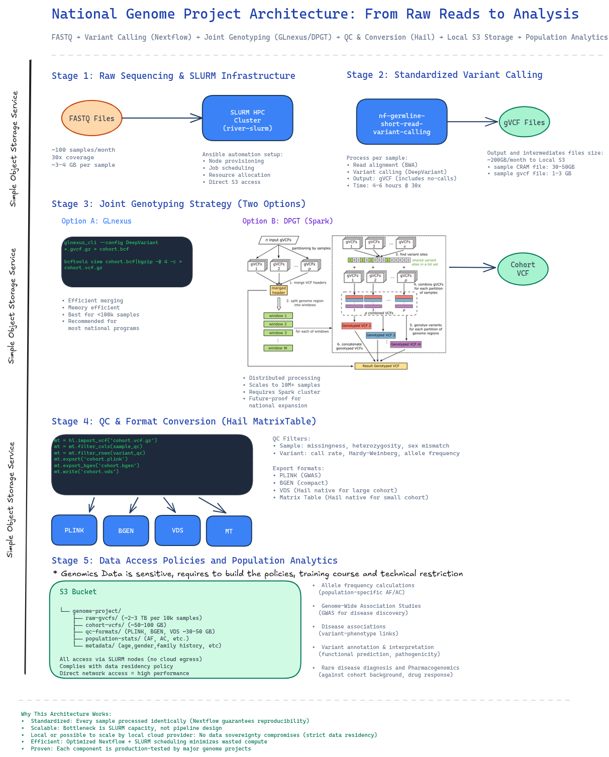
Figure 2: End-to-end architecture showing data flow from raw sequencing through population analytics, with concrete tools and storage at each stage.
2.1. Stage 1: Core Infrastructure with SLURM HPC Cluster
- Proof of Concept for Building the Typical SLURM Clutser Bioinformatics Analysis: https://github.com/gianglabs/river-slurm
The foundation is a high-performance computing cluster managed by SLURM.
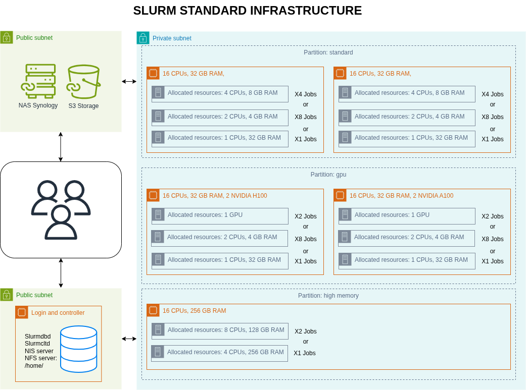
Figure 3: SLURM HPC cluster and Simple Object Storage S3 architecture
Key setup:
- ansible automation: Use the proven river-slurm Ansible playbook to configure SLURM from scratch
- Automatic node provisioning and job scheduling
- Resource allocation policies tuned for bioinformatics workloads
- Network and storage integration
- Local compute: All processing happens on-site, no data egress to cloud
- Direct S3 access: SLURM nodes can directly read/write to local/domestic S3 storage
Why SLURM?
- It's the industry standard for HPC. It scales from dozens to thousands of nodes, handles complex job dependencies, and integrates seamlessly with bioinformatics tools.
- Distributed system can be run on top of SLURM for scaling the bioinformatics analysis
- Easy to integrate to the domestic cloud provider
2.2. Stage 2: Standardized Variant Calling
- Proof of Concept for Short Read Germline Variant Calling: https://github.com/gianglabs/nf-germline-short-read-variant-calling
- The common modules and subworkflows are developed and maintained with customization at: https://github.com/gianglabs/nf-modules
Every genome must go through identical variant calling logic. This is non-negotiable for cohort analyses.
The pipeline: nf-germline-short-read-variant-calling
- Built on Nextflow for reproducibility and portability
- Carefully benchmarked for accuracy and efficiency
- Benchmarked to find the best choice for the large scale variant calling genomics project
- Optimized to run efficiently on SLURM clusters
- Outputs individual gVCF files (genome VCF format—raw variants per sample)
Why gVCF? It includes not just called variants, but also "confident no-calls" at each genomic position. This is crucial for joint genotyping later—without it, you lose information about coverage depth and genotype quality.
Scale: Processing 100 samples/month at 30x coverage:
- Individual variant calling: ~4-6 hours per genome on a standard node. Faster with GPU for variant calling using DeepVariant
- Parallelizable across SLURM queue
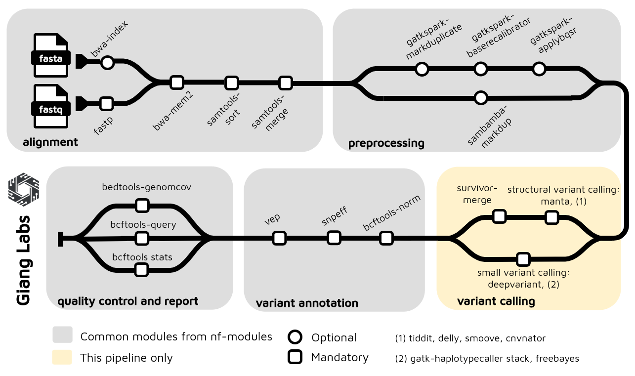 Figure 4: The nextflow pipeline for short read variant calling using Illumina platform, optimized for 30X WGS. The pipeline is integrated with nf-modules where it standardizes to share the common components between pipelines
2.3. Stage 3: Joint Genotyping — Cohort Integration
- Proof of Concept for Joint Genotyping using GLnexus: https://github.com/gianglabs/gkit/tree/main/glnexus
- Proof of Concept for Joint Genotyping using DPGT: https://github.com/gianglabs/gkit/tree/main/dpgt
- Spark on SLURM that DPGT can submit job to https://github.com/gianglabs/gkit/tree/main/spark-on-slurm
After variant calling, you have a thousands of individual gVCF files and each sample called independently. But independent calling is not enough for population-scale genomics. You must combine them into a cohort VCF using joint variant calling.
Example:
sample A:
- chr1:1000 A>G (variant detected)
sample B:
- chr1:1000 no variant detected
while sample B may have these artifacts:
- Maybe Sample B had low coverage
- Maybe variant signal was weak
- Variant may actually exist but missed
Two proven options:
Option A: GLnexus (Efficient, Recommended for <100k samples)
- Joint calling based on the region of bed file can be used to compute parrallelly
- Flanking regions are required mainly because variant representation and normalization can extend beyond the target window, especially for indels and complex variants.
# GLnexus merges gVCFs into a cohort VCF
glnexus_cli --config DeepVariant_h37 --bed <bed file> *.gvcf.gz > cohort.bcf
bcftools view cohort.bcf -O z > cohort.vcf.gz
- Dramatically faster than GATK GenotypeGVCFs
- Excellent quality for medium-scale cohorts
- Memory efficient (can run on modest hardware)
Option B: DPGT with Spark (Distributed, Scales to Millions)
#!/bin/bash
# DPGT runner for joint genotyping cohort VCF

set -euo pipefail

PROJECT_ROOT="$(cd "$(dirname "${BASH_SOURCE[0]}")/.." && pwd)"
BUILD_LIB_PATH="${PROJECT_ROOT}/build/lib"
DPGT_JAR="${PROJECT_ROOT}/DPGT/target/dpgt-1.3.2.0.jar"

# Defaults (override with env vars if needed)
INPUT_LIST="${INPUT_LIST:-${PROJECT_ROOT}/cohort_vcf/1KGP/gvcf_input.list}"
REFERENCE_FASTA="${REFERENCE_FASTA:-${PROJECT_ROOT}/reference/Homo_sapiens_assembly38.fasta}"
OUTPUT_DIR="${OUTPUT_DIR:-${PROJECT_ROOT}/cohort_vcf/1KGP/results}"
TARGET_REGION="${TARGET_REGION:-chr12:111760000-111763759}"
JOBS="${JOBS:-4}"
ALLOW_OVERWRITE="${ALLOW_OVERWRITE:-0}"

echo "================================"
echo "DPGT Cohort VCF Runner"
echo "================================"
echo ""

# Check prerequisites
echo "Checking prerequisites..."
if [ -z "$DPGT_JAR" ] || [ ! -f "$DPGT_JAR" ]; then
    echo "ERROR: DPGT JAR not found at $DPGT_JAR"
    echo "Run 'make build' to compile DPGT first"
    exit 1
fi

if [ ! -f "$BUILD_LIB_PATH/libcdpgt.so" ]; then
    echo "ERROR: libcdpgt.so not found at $BUILD_LIB_PATH"
    echo "Run 'make build-cpp' to compile C++ libraries"
    exit 1
fi

if [ ! -f "$INPUT_LIST" ]; then
    echo "ERROR: input list not found: $INPUT_LIST"
    echo "Create it with one gVCF path per line (3-sample trio supported)."
    echo "Example existing list: ${PROJECT_ROOT}/gvcf_input.list"
    exit 1
fi

if [ ! -f "$REFERENCE_FASTA" ]; then
    echo "ERROR: reference fasta not found: $REFERENCE_FASTA"
    exit 1
fi

if [ -d "$OUTPUT_DIR" ] && [ "$(ls -A "$OUTPUT_DIR" 2>/dev/null || true)" != "" ]; then
    if [ "$ALLOW_OVERWRITE" = "1" ]; then
        echo "Output exists. Removing: $OUTPUT_DIR"
        rm -rf "$OUTPUT_DIR"
    else
        echo "ERROR: output directory exists and is not empty: $OUTPUT_DIR"
        echo "Set ALLOW_OVERWRITE=1 or choose another OUTPUT_DIR"
        exit 1
    fi
fi

echo "DPGT JAR: $DPGT_JAR"
echo "C++ Library: $BUILD_LIB_PATH/libcdpgt.so"
echo "Input List: $INPUT_LIST"
echo "Reference: $REFERENCE_FASTA"
echo "Output Dir: $OUTPUT_DIR"
echo "Region: $TARGET_REGION"
echo ""
echo "Note: default region is a small smoke-test interval."
echo ""

# Runtime environment
export LD_LIBRARY_PATH="$BUILD_LIB_PATH:${LD_LIBRARY_PATH:-}"

echo "Running DPGT joint genotyping..."
echo ""

# Some environments need explicit local filesystem implementations for Spark/Hadoop
java \
  -Dspark.hadoop.fs.file.impl=org.apache.hadoop.fs.LocalFileSystem \
  -Dspark.hadoop.fs.AbstractFileSystem.file.impl=org.apache.hadoop.fs.local.LocalFs \
  -cp "$DPGT_JAR" \
  org.bgi.flexlab.dpgt.jointcalling.JointCallingSpark \
  -i "$INPUT_LIST" \
  -r "$REFERENCE_FASTA" \
  -o "$OUTPUT_DIR" \
  -j "$JOBS" \
  -l "$TARGET_REGION" \
  --local

echo ""
echo "Run complete."
echo "Output files in: $OUTPUT_DIR"
find "$OUTPUT_DIR" -maxdepth 1 -type f -name "result*.vcf.gz" -print || true
- Built on Apache Spark for distributed computing
- Linear scaling with sample count
- Better for national programs planning billion-scale expansion
- Requires Spark cluster (can run on same SLURM infrastructure)
Output: A single cohort.vcf.gz with all samples and all variants. For ~1000 samples project, it can be 200-500GB (it is depended on the diversity of variants and samples)
2.4. Stage 4: Cohort QC and Format Conversion (Hail)
- Proof of Concept for Hail: https://github.com/gianglabs/gkit/hail
- Hail should be run on the Spark Cluster on the top of SLURM: https://github.com/gianglabs/gkit/spark-on-slurm
The raw cohort VCF isn't analysis-ready. It needs QC and must be converted to efficient formats. QC should be adjusted according to the quality of the ingested data
Using Hail's MatrixTable:
# Load cohort VCF into Hail
mt = hl.import_vcf('cohort.vcf.gz')

# Sample-level QC
mt = mt.filter_cols(hl.agg.count_where(mt.GT.is_non_ref()) > 100)

# Variant-level QC
mt = mt.filter_rows(hl.agg.count_where(mt.GT.is_non_ref()) > 0)

# Export to multiple formats for different tools
mt.export('cohort.plink')      # PLINK format for association studies
mt.export_bgen('cohort.bgen')  # BGEN format (more efficient)
mt.write('cohort.vds')         # Hail VDS (best for Hail)
Export formats for different use cases:
- PLINK (.bed/.bim/.fam): Standard format for GWAS, linkage analysis
- BGEN: Compact binary format, efficient for large cohorts
- VDS (Hail format): Native Hail format, fastest for downstream Hail analyses
- Hail MatrixTable: In-memory representation for interactive analysis
QC filtering removes:
- Samples with excessive missing data
- Samples with unexpected heterozygosity or sex mismatches
- Variants with low call rates or Hardy-Weinberg violations
- Variants with extreme allele frequency outliers
2.5. Stage 5: Long-term Data Storage & Access Policies
Data Sovereignty Strategy: Rather than building on-premises storage infrastructure, partner with a domestic S3 provider (cloud or government-backed) for long-term data residency. This keeps data in-country while avoiding large capital investment in storage hardware.
Nowadays, the data should be accessed via the data platform where users need to:
- Learn and pass the training courses where users are allowed only to use the data for analysis on the controlled platform. They are not allowed to download the data or intermediate data that can reveal/identify personality.
- Not only restrict by policies, the data platform should be able to restrict users according to the data platform architect
Architecture:
The system architecture consists of:
- SLURM Cluster (on-premises) with direct S3 access via local network peering
- S3 Bucket (domestic provider) containing:
- Raw gVCFs (archived, immutable, 10 years)
- Cohort VCFs (versioned releases)
- Cohort MatrixTables (Hail-native)
- Final analytics formats (PLINK/BGEN/VDS/MT)
Why this partnership model?
- Data sovereignty: Genomic data never leaves the country. Domestic S3 provider ensures local data residency
- No capital burden: Pay-as-you-go storage
- Scalability: Expand from 10TB to 100TB+ without hardware refresh
- Performance: Direct network access from SLURM cluster (local peering, not internet)
- Compliance: Meets strict data residency policies and regulatory requirements
- Integration: Nextflow, Hail, and SLURM all have native S3 support
- Longevity: Partner contract ensures data availability beyond project timeline (5-10 years)
Long-term value: After the 1k-sample project completes, this S3 infrastructure remains available for future extensions (multi-omics storage, disease cohort data, long-term archival)
3. Design Principles
3.1. Standardization as the Foundation
Without CI/CD integration, "standardization" is just a claim, not a guarantee.
- No CI/CD = manual testing = inconsistent results across developers/environments
- With CI/CD = automated testing = identical results every time, on HPC or Cloud
Every sample must go through identical processing—this is non-negotiable for population-scale analyses.
Why standardization matters:
- Reproducibility: Same input data + same pipeline = same results every time
- Quality assurance: Systematic issues caught early and applied uniformly across all samples
- Cross-cohort comparisons: Different batches and timepoints can be compared without systematic bias
- Joint analyses: Cohort-wide statistics are only valid when all samples processed identically
Implementation:
- Use Nextflow for pipeline versioning and reproducibility
- gVCF format enforces standardized output across all samples
- Version control (Github, Gitlab, Gitea, etc): Track pipeline versions, reference genome versions, annotation database versions
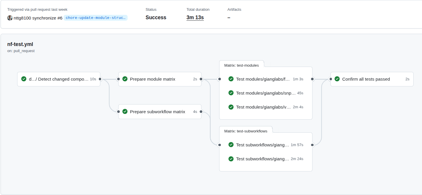
Figure 5: The CI/CD on the nf-modules where it shows the concepts to ensure that the common patterns (modules, subworkflows), can be identical, reproducible and reused accross multiple pipelines.
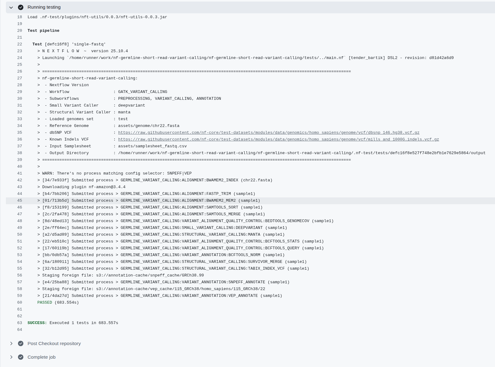 Figure 6: The CI/CD on the nf-germline-short-read-variant-calling where the identical inputs should create the same output files, the workflows also be able to deploy on HPC, Cloud
3.2. Scalability Through Region-Based Parallelization
Joint variant calling works on the entire cohort simultaneously, not sample-by-sample. The key to scaling is splitting the genome into smaller, independent regions (windows) and processing all samples together within each region in parallel.
The Parallelization Strategy:
- All samples in each region: For region 1, call variants across ALL samples simultaneously; for region 2, call variants across ALL samples; etc.
- Region-based parallelization: Each genomic region runs on a separate SLURM job, enabling horizontal scaling
- Failure isolation: If one region fails, you only re-run that region—not the entire genome for all samples
Bed File Strategy (Chromosome-Based with Intervals):
For small-to-medium cohorts (<10k samples): Use simple chromosome-based BED files (one per chromosome):
- chr1.bed covering chr1:1-248956422
- chr2.bed covering chr2:1-242193529
- ... and so on for all 22 autosomes
- chrX.bed and chrY.bed for sex chromosomes
For large cohorts (>10k samples): Split each chromosome into 100kb intervals for finer-grained parallelization:
- chr1_region_1.bed: chr1:1-100000
- chr1_region_2.bed: chr1:100001-200000
- chr1_region_3.bed: chr1:200001-300000
- ... continuing across all chromosomes with thousands of regions
Why this interval-based approach scales:
- Memory efficiency: Each region holds only ~100kb of genomic data per sample, not entire chromosomes
- Job parallelization: 22 chromosomes × 24,000 intervals = 528,000 potential SLURM jobs (realistic for 50k+ sample cohorts)
- Failure recovery: Failed region only requires re-running 100kb interval, not entire chromosome
- SLURM queue optimization: Small jobs (100kb regions) fit better into queue scheduling than large jobs
Example workflow with GLnexus (chromosome-based for <10k):
# For each chromosome in parallel:
glnexus_cli --config DeepVariant_h37 \
  --bed chr1.bed \
  sample1.gvcf.gz sample2.gvcf.gz ... sampleN.gvcf.gz \
  > cohort_chr1.bcf

# For chr2, chr3, etc. (run in parallel across SLURM cluster)

# Merge all chromosomal BCF files
bcftools concat cohort_chr*.bcf -O z > cohort.vcf.gz
Example for large cohorts (interval-based for >10k):
# For each 100kb interval in parallel:
glnexus_cli --config DeepVariant_h37 \
  --bed chr1_region_1.bed \
  sample1.gvcf.gz sample2.gvcf.gz ... sample10000.gvcf.gz \
  > cohort_chr1_region_1.bcf

# Across all regions simultaneously (SLURM schedules thousands of jobs)

# Final merge (can be done hierarchically: chr1 regions → chr1.bcf, then merge all chr*.bcf)
bcftools concat cohort_chr*_region_*.bcf -O z > cohort.vcf.gz
Why this is fundamentally different from:
- ❌ Single-sample variant calling: Cannot be used for joint genotyping (loses population information)
- ❌ Whole-genome per-cohort in one job: No parallelization, no failure recovery, memory explosion at scale
- Region-based cohort calling: Scales linearly, fails gracefully, maximizes SLURM parallelization
3.3. Data Storage and Sharing
For the data storage, it should standardizes to store the needed data only:
- Data should be stored and grant the access with the approriate permission
- BAM,CRAM file should be kept where they can restore to the original format (fastq) while save storage and be the inputs for many tools to extract more informations from the data
- Hail Matrix Table, VDS, Plink, Bgen are the pre-processed high-quality data can be ready for analysis.
- User do not need to reingest data that repeat the pre-process and quality control step
Table 1: Pipelines and bioinformatics tools utilized in genomic resources in the national biobank
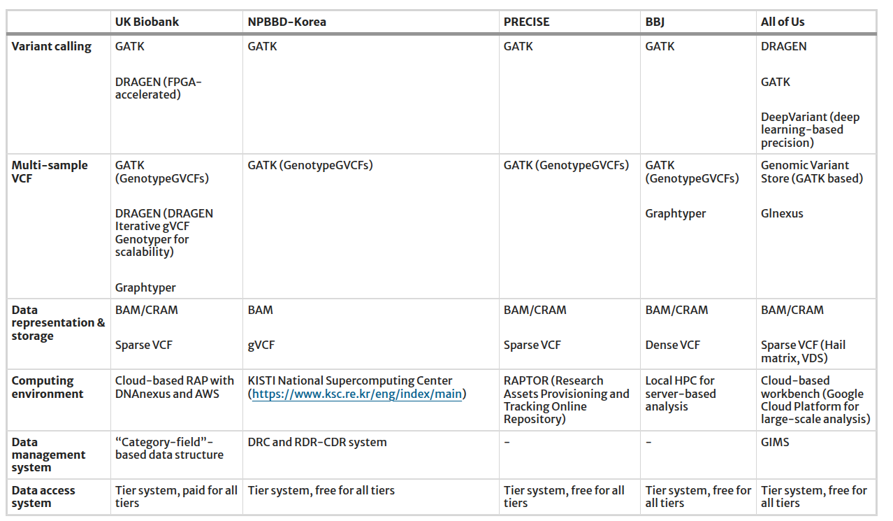
Reference: https://link.springer.com/article/10.1186/s44342-025-00040-9
Don't just store raw data; design storage tiers for downstream analysis from the start.
Three-Tier Storage:
| Tier | Format | Purpose | Size (10k samples) |
|---|---|---|---|
| Raw | gVCF | Source data, immutable, archival | 2-3 TB |
| Processed | Cohort VCF | QC baseline, joint-called, version-controlled | 50-100 GB |
| Analytics | PLINK, BGEN, VDS | Analysis-ready, indexed, compressed | 30-50 GB |
Table 2: Three-tier storage architecture for genome project data
Analytics formats enable different use cases:
- PLINK: GWAS, linkage analysis, PCA (de facto standard in genetics)
- BGEN: Compact binary format, excellent for large-scale population studies
- VDS (Hail): Columnar format, best for Hail analytics and machine learning pipelines
3.4. Federated Governance and Multi-Institutional Collaboration
Most national genomic projects involve multiple hospitals, universities, and research centers contributing samples.
Federated Model:
- Each institution contributes samples independently
- Central joint genotyping ensures consistency: all samples called together, not separately per institution
- Shared infrastructure: multiples SLURM cluster, multiples S3 storage while centralize data analytics platform
Privacy-Preserving Architecture:
- Raw data: restricted access (only institution that contributed it)
- QC'd cohort data: institutional researchers + project leadership
- Aggregated statistics (allele frequencies, QC metrics): publicly shared (no individual-level data)
- Compute-to-data: Analysis runs on the secure cluster; results exported, not raw data
Role-Based Access Control:
Raw gVCF data
  ├─ Accessible to: Original institution + data stewards
  └─ Access: read-only, audit-logged

Cohort VCF (QC'd)
  ├─ Accessible to: Project researchers
  └─ Access: for analysis with ethics approval

Public allele frequencies
  ├─ Accessible to: General public
  └─ Download from website
This design principle enables nations to collaborate across institutions while maintaining strict data governance and participant privacy.
4. Infrastructure Layer & Implementation Roadmap
Building a national genome project requires careful sequencing of phases. This section outlines both the infrastructure requirements and a realistic implementation timeline.
4.1. Infrastructure Requirements Overview
A national genome project infrastructure stack consists of three core layers:
| Layer | Component | Technology | Purpose |
|---|---|---|---|
| Compute | HPC Cluster | SLURM + compute nodes | Variant calling, joint genotyping, analytics |
| Storage | Object Storage | S3-compatible (on-premises) | gVCFs, VCFs, analytics formats |
| Analytics | Data Platform | Hail, Python, Spark | Population statistics, GWAS, QC |
Table 3: Core infrastructure layers for national genome project
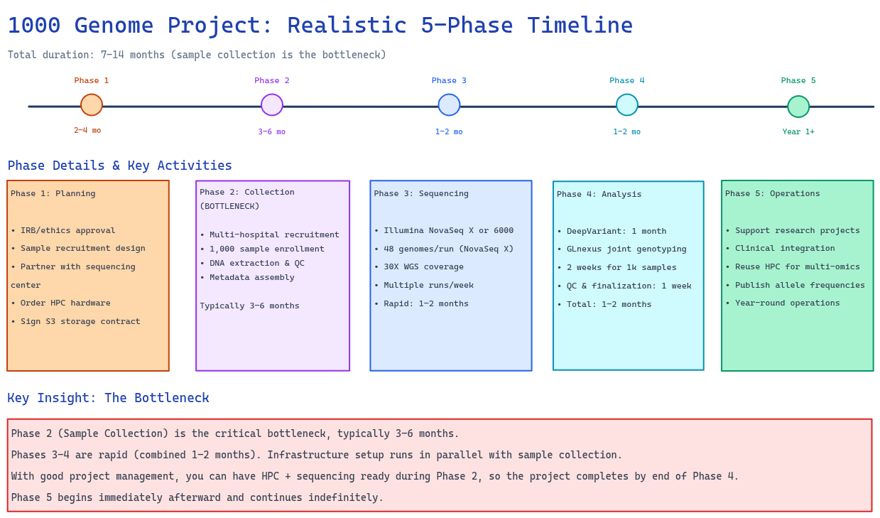 Figure 7: Realistic 6–12 month implementation roadmap showing all five phases. Key insight: Phase 2 (Sample Collection) is the bottleneck (3–6 months). Phase 3 (Sequencing) and Phase 4 (Variant Calling + QC) are rapid (1–2 months each). Infrastructure setup runs in parallel with sample collection.
4.2. Phase 1: Planning & Ethics (2–4 months)
Goals:
- Secure institutional approvals (IRB/ethics)
- Design sample recruitment strategy
- Establish sequencing partnerships
- Begin infrastructure procurement
Timeline:
- IRB/ethics approval: 1–2 months
- Sample recruitment design & partnership agreements: 1–2 months
- Parallel: Order HPC hardware and establish S3 partnership contracts
Outcomes at End of Phase 1:
- IRB/ethics approval obtained
- Recruitment strategy finalized
- Sequencing capacity confirmed (partner with sequencing center or in-house)
- HPC hardware ordered (delivery 4–8 weeks)
- S3 partnership contract signed
4.3. Phase 2: Sample Collection (3–6 months)
Goals:
- Recruit and enroll 1,000 participants
- Perform DNA extraction
- Establish data governance protocols
Timeline:
- Multi-hospital recruitment: 3–6 months (usually the slowest phase)
- DNA extraction & quality control: Parallel to recruitment
- Cohort metadata assembly: Concurrent
Key Challenge: Sample collection is typically the bottleneck. Plan for:
- Hospital coordination across multiple sites
- Participant compliance and scheduling
- DNA quality control (ensure >95% pass-through)
- Metadata standardization
Outcomes at End of Phase 2:
- 1,000 samples collected, extracted, and QC'd
- Metadata database established
- Samples ready for sequencing
4.4. Phase 3: Sequencing (1–2 months)
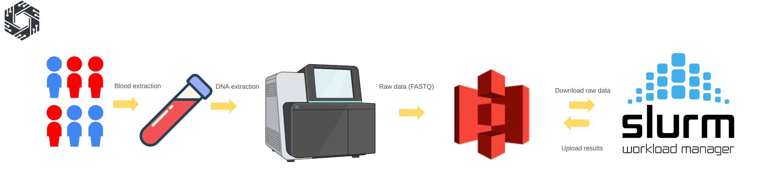
Figure 8: Sequencing procedure: Blood samples are collected from participants and genomic DNA is extracted using standard laboratory protocols. The DNA is then prepared for sequencing and processed on high-throughput platforms, generating raw sequencing data in FASTQ format. The raw data is uploaded to object storage such as Amazon S3 or an S3-compatible partner. The HPC system downloads the data from S3, performs alignment and variant calling, and uploads the processed outputs back to S3 for long-term storage and downstream population analysis.
Goals:
- Sequence all 1,000 samples at 30X WGS depth
- Deliver FASTQ files to HPC cluster
- Begin variant calling immediately as data arrives
HPC Cluster Setup (Parallel to Sequencing):
Reference: river-slurm Ansible playbook
Minimum viable cluster:
- 1 head node (Slurm controller, login node)
- 4-8 compute nodes (2-socket, 32-64 CPU each)
- 100TB local SSD for scratch space
- 1Gbps network connectivity
Optional enhancement (for faster variant calling):
- 2 GPU nodes with NVIDIA GPU (for DeepVariant acceleration)
- Reduces per-sample variant calling from 4-6 hours (CPU-only) to 1-2 hours per sample
- Optional optimization (not required for 1k-sample target)
Using Ansible for Infrastructure Automation:
# Deploy entire SLURM cluster from scratch
ansible-playbook -i inventory.ini cluster_slurm.yml

# Validates:
- 1. All nodes can submit/run jobs
- 2. Job scheduling policies working
- 3. Network connectivity stable
Domestic S3 Storage Partnership (Initiated)
- Industry-standard storage: Object storage such as Amazon S3, Google Cloud Storage, or Azure Blob Storage or Local compatible S3 provider is widely used across industries, ensuring scalability, compatibility, and long-term sustainability beyond bioinformatics use cases.
- High availability requires dedicated expertise: Population genomics projects generate hundreds of TB to PB-scale data. Maintaining high availability, throughput, backup, and security requires a dedicated infrastructure team, which increases operational complexity.
- Reduced operational cost and complexity: Partnering with an S3 provider shifts infrastructure management to experienced teams, reducing maintenance overhead and allowing the project to focus on analysis and scientific outcomes.
Using the external S3 provider is a feasible approach
Options:
- Commercial domestic cloud provider (with local data residency)
- Government-backed infrastructure (if available in your country)
- Academic cloud partnership (university data center)
Key requirements:
- Data never leaves the country (sovereignty requirement)
- On-premise SLURM nodes have direct network access (low latency)
- Contract negotiated for 5-10 year commitment
- Scalable from this project while opening the possibility to extend the storage volume
Quality Control For Raw Data
After sequencing, the raw FASTQ data should undergo quality control to ensure it is suitable for downstream analysis. This step typically includes checking sequencing quality scores, read length distribution, GC content, adapter contamination, and duplication levels using tools such as FastQC and MultiQC.
Samples that do not meet quality thresholds may require re-sequencing or additional preprocessing such as adapter trimming and filtering. Performing quality control at this stage ensures that the data is reliable and ready for subsequent alignment and variant calling steps.
Outcomes at End of Phase 3:
- All 1,000 samples sequenced (FASTQ files delivered)
- FASTQ files transferred to HPC cluster and archived in S3
- Ready for variant calling in Phase 4
4.5. Phase 4: Variant Calling + QC (1–2 months)
Goals:
- Call variants on all 1,000 samples using DeepVariant
- Perform joint genotyping with GLnexus
- Complete cohort QC and finalization
Variant Calling Pipeline (Parallel to Sequencing):
Deploy nf-germline-short-read-variant-calling https://github.com/gianglabs/nf-germline-short-read-variant-calling
Using DeepVariant for high-accuracy variant calling:
- Per-sample variant calling: 4-6 hours (CPU-only) 1-2 hours (with GPU acceleration)
- Chromosome-based parallelization: 22 concurrent jobs
Timeline for 1,000 samples:
- With 4-8 CPU nodes: ~1-2 weeks for all gVCF generation
- With optional 2 GPU nodes: ~1 week for all gVCF generation
Joint Genotyping:
GLnexus performs joint genotyping by:
- Combining all 1,000 gVCFs into a cohort VCF
- Using chromosome-based processing with 22 parallel jobs
- Completing in 2–5 days (depending on variant density)
- Producing a single cohort VCF with all variants
QC + Cohort Assembly:
After joint genotyping, perform quality control checks:
- Sample-level QC: contamination, depth, relatedness
- Variant-level QC: allele frequency distribution, Hardy-Weinberg equilibrium
- Population structure analysis: PCA
- Prepare final release cohort VCF
Timeline: approximately 1 week for QC and finalization
Total Phase 4 Duration: 1–2 months
- Variant calling: 1–2 weeks
- Joint genotyping: 2–5 days
- QC & finalization: 1 week
- Combined: 1–2 months total
Outcomes at End of Phase 4:
- All 1,000 samples processed through variant calling
- 1,000 high-quality gVCF files generated
- Cohort VCF finalized (joint genotyping complete)
- Population-level QC passed
- Ready for analytics and research
4.6. Phase 5: Operations & Research Enablement (Year 1+)
Goals:
- Establish steady-state operations
- Enable population-level research
- Support clinical diagnostics and precision medicine
Infrastructure Maturity:
- Maintain 4-8 compute nodes (core infrastructure)
- Optional 2 GPU nodes for accelerated variant calling
Key Reuse Opportunity: This infrastructure was built for 1k-genome analysis, but can be repurposed:
- Multi-omics processing (proteomics, metabolomics, RNA-seq)
- Rare disease interpretation pipelines
- Clinical genomics workflows
- Advanced bioinformatics research platform
Capacity at 1k-sample scale:
- GWAS analyses: minutes to hours
- Variant annotation pipelines: hours
- Population statistics: minutes
- Spare capacity: available for other research
Analytics Platform: Hail MatrixTable (for population analytics):
- All 1,000 samples + variants in single analysis object
- Per-sample QC: compute ancestry, relatedness, sample-specific statistics
- Per-variant QC: allele frequency distribution, population structure
- Rapid queries: filter by allele frequency, population, phenotype
Research enablement:
- Export to PLINK for GWAS
- Export to BGEN for imputation studies
- Direct analysis via Hail Batch for distributed computing
Data Access & Governance: Domestic S3 Storage (Long-term):
- Established contract: 5-10 year commitment
- Data residency: All data stays in-country
- Pay-as-you-grow model: ~$0.02-0.05/GB/month
- Direct SLURM access: low-latency queries
Data access policies:
- Researchers access data via controlled analytics platform
- Training required before data access
- Audit trails for all data access
- No raw data downloads (aggregate statistics only)
Outcomes at End of Phase 5:
- Production-grade operations established
- Research projects supported
- Clinical integration pathways clear
- Infrastructure reusable for future projects
4.7. Overall Timeline Summary
Total Project Duration: 6–12 months (realistic range accounting for sample collection bottleneck)
| Phase | Activity | Duration | Bottleneck |
|---|---|---|---|
| Phase 1 | Planning & Ethics | 2–4 months | IRB approval |
| Phase 2 | Sample Collection | 3–6 months | Multi-hospital recruitment |
| Phase 3 | Sequencing | 1–2 months | Sample delivery speed |
| Phase 4 | Variant Calling + QC | 1–2 months | Computational throughput |
| Phase 5 | Operations & Research Enablement | Year 1+ | Ongoing |
Table 4: Project timeline summary with phase durations and bottlenecks
Key Insight: The critical path is Phase 2 (Sample Collection), which typically takes 3-6 months. Phases 3 and 4 are rapid (1–2 months each). Infrastructure (Phase 1 planning and Phase 3 implementation) runs in parallel with sample collection.
4.8. Critical Success Factors
Technical:
- Robust variant calling (validated benchmarking)
- Reliable joint genotyping (tested thoroughly)
- Automated QC (catches errors before publication)
- CI/CD integration (ensures reproducibility)
Organizational:
- Dedicated team (at least 2-3 full-time staff, stable)
- Clear governance (who decides on data access, pipeline changes)
- Institutional buy-in (hospital systems, university commitment)
- Sustainable funding (multi-year commitment, not grant-dependent)
Strategic:
- Population engagement (transparent about data use)
- Research partnerships (early collaboration with universities)
- Clinical integration (demonstrate direct patient benefit)
- International standards (align with 1000 Genomes, GA4GH, etc.)
4.9. Risk Mitigation & Contingencies
Risk: Pipeline bugs causing systematic errors in 1k samples
- Mitigation: Comprehensive CI/CD testing; region-based processing with checkpoints; ability to re-run any region
Risk: Data loss or corruption
- Mitigation: Multi-site backup; immutable gVCFs archived; version control on all code/configs
Risk: Key staff turnover
- Mitigation: Documentation, runbooks, training; knowledge transfer; open-source code (no vendor lock-in)
Risk: Regulatory changes affecting data sharing
- Mitigation: Privacy-by-design (local storage, role-based access); clear consent forms; regular legal review
Risk: Funding interruption
- Mitigation: Demonstrate research value early; publish results; engage stakeholders; seek multi-year commitments
5. Variant Calling & Joint Genotyping
Detailed implementation guides for variant calling and joint genotyping are covered in our dedicated blog series:
- Variant Calling: See our comprehensive series on nf-germline-short-read-variant-calling pipeline
- Joint Genotyping: Detailed technical walkthroughs for GLnexus and DPGT implementations
- Benchmarking: Performance comparisons and optimization techniques
This blog focuses on the architecture-level decisions and ecosystem integration rather than pipeline internals. Refer to the dedicated blogs for implementation details, code walkthroughs, and troubleshooting.
6. Cohort Analytics Layer (Hail) — Enabling "Open Work" for Researchers
- The exported data can support multiple research purposes, including integration with EHR and external datasets.
- The following sections are for illustration only; practical analyses typically require more extensive effort.
6.1 Why the Analytics Layer Matters
The true value of a national genome project emerges in the "open work" phase—when researchers can freely query your 1k-sample cohort to answer scientific questions. This requires more than just storing raw genotypes. You need:
- Multiple export formats (PLINK, BGEN, VDS) so different research tools can work efficiently
- Population statistics (allele frequencies, ancestry information, phenotype summaries) accessible to all researchers
- Quality-controlled, analysis-ready data that researchers can trust
- Fast query infrastructure (MatrixTable, HailQL) for exploratory analysis
The analytics layer is the difference between "we have genome data" and "researchers can use our genome data."
This section shows how to build that infrastructure.
6.2. From Raw VCF to Research-Ready Data
Once you have a cohort VCF with all samples jointly-called, the next critical step is transforming it into analysis-ready formats and populating metadata for QC and filtering.
Why Hail for this layer:
- Scalable: Processes cohort VCFs with 100k+ samples efficiently
- Flexible: Export to PLINK, BGEN, VDS, or keep as MatrixTable
- Production-ready: Used by major biobanks (UK Biobank, gnomAD, etc.)
- Analytics integration: Built-in for GWAS, burden tests, population statistics
6.3. Hail MatrixTable Workflow
Load cohort VCF:
import hail as hl

# Import cohort VCF into Hail MatrixTable
mt = hl.import_vcf('s3://genome-project/cohort.vcf.gz')

# MatrixTable structure:
# - Rows: Variants (SNPs, indels, etc.)
# - Columns: Samples
# - Entries: Genotypes (0/0, 0/1, 1/1, ./.)
Add annotations:
# Variant-level annotations
mt = hl.vep(mt)  # Functional prediction
mt = mt.annotate_rows(
    gnomad_af = gnomad.rows()[mt.row_key].AF,
    clinvar_sig = clinvar.rows()[mt.row_key].significance
)

# Sample-level annotations (sex, ancestry, phenotype)
mt = mt.annotate_cols(
    sex = sample_meta[mt.col_key].sex,
    ancestry = sample_meta[mt.col_key].ancestry,
    case_status = sample_meta[mt.col_key].phenotype
)
QC filtering:
# Sample QC
sample_qc = hl.sample_qc(vds)
mt = mt.annotate_cols(qc = sample_qc[mt.col_key])

# Filter based on QC metrics
mt = mt.filter_cols(
    (mt.qc.n_het > 0) &  # Has heterozygous calls
    (mt.qc.dp_mean > 30) &  # Average depth >30x
    (mt.qc.r_ti_tv > 2.0)  # Ti/Tv ratio normal
)

# Variant QC
mt = mt.filter_rows(hl.agg.count_where(mt.GT.is_non_ref()) > 0)
Export to analysis-ready formats:
# PLINK format (for GWAS)
hl.export_plink(mt, 'cohort.bed', 'cohort.bim', 'cohort.fam')

# BGEN format (compact, efficient)
hl.export_bgen(mt, 'cohort.bgen')

# VDS (Hail native, best for future Hail analyses)
mt.write('s3://genome-project/cohort.vds', overwrite=True)
6.4. Population-Level Statistics
Calculate allele frequencies:
# Global allele frequencies
mt = mt.annotate_rows(
    allele_freq = hl.agg.allele_stats(mt.GT).AF,
    ac = hl.agg.count_where(mt.GT.is_non_ref()),
    an = hl.agg.count() * 2
)

# Ancestry-stratified frequencies (if multi-population)
mt = mt.annotate_rows(
    freq_by_ancestry = hl.agg.collect_as_dict(
        mt.ancestry,
        hl.agg.allele_stats(mt.GT).AF
    )
)
Population genetics calculations:
# Hardy-Weinberg equilibrium
mt = mt.annotate_rows(
    hwe = hl.hardy_weinberg_test(
        hl.agg.count_where(mt.GT == hl.call(0, 0)),
        hl.agg.count_where(mt.GT == hl.call(0, 1)),
        hl.agg.count_where(mt.GT == hl.call(1, 1))
    )
)

# Principal Component Analysis (population structure)
pc_eigenvalues, pc_scores, pc_loadings = hl.pca(
    mt.GT.n_alt_alleles(),
    k=20,
    compute_loadings=True
)
6.5. Variant Annotation Pipeline
Integrate external resources:
# ClinVar pathogenicity
clinvar = hl.read_table('gs://hail-datasets/clinvar.ht')
mt = mt.annotate_rows(
    clinvar_sig = clinvar.rows()[mt.row_key].significance
)

# gnomAD frequencies (population reference)
gnomad = hl.read_table('gs://hail-datasets/gnomad.ht')
mt = mt.annotate_rows(
    gnomad_ac = gnomad.rows()[mt.row_key].AC,
    gnomad_af = gnomad.rows()[mt.row_key].AF
)

# CADD scores (variant effect prediction)
cadd = hl.read_table('path/to/cadd.ht')
mt = mt.annotate_rows(
    cadd_score = cadd.rows()[mt.row_key].score
)
Create interpretable variant categories:
# Flag likely pathogenic variants
mt = mt.annotate_rows(
    is_likely_pathogenic = (
        (mt.clinvar_sig == 'pathogenic') |
        ((mt.cadd_score > 30) & (mt.gnomad_af < 0.01))
    ),
    is_rare = mt.gnomad_af < 0.01,
    is_common = mt.gnomad_af > 0.05
)
6.6. Rare Disease Interpretation & Diagnosis
Using cohort as background reference:
# For each rare disease sample, find matching variants in cohort
# Example: Exome analysis with population context

rare_disease_mt = hl.read_matrix_table('rare_disease_samples.vds')

# Annotate with cohort allele frequencies
rare_disease_mt = rare_disease_mt.annotate_rows(
    cohort_af = mt.rows()[rare_disease_mt.row_key].allele_freq,
    cohort_ac = mt.rows()[rare_disease_mt.row_key].ac
)

# Prioritize rare variants (absent or very rare in cohort)
rare_disease_mt = rare_disease_mt.filter_rows(
    (rare_disease_mt.cohort_ac < 5) |  # <5 people in cohort
    hl.is_missing(rare_disease_mt.cohort_af)  # Not in cohort at all
)
6.7. Example Research Projects ("Open Work")
This is where the value of your genome project becomes visible. Once the infrastructure is ready, researchers can immediately begin:
Example 1: Genome-Wide Association Study (GWAS)
# Researcher has 1k individuals, 500 with Type 2 Diabetes, 500 without
# Goal: Find variants associated with diabetes in your population

from hail.methods import linear_regression_rows

# Load PLINK format
mt = hl.read_table('cohort.plink')

# Fit linear regression: genotype ~ diabetes status
mt = mt.annotate_rows(
    beta = linear_regression_rows(
        y=mt.phenotype.diabetes,
        x=mt.GT.n_alt_alleles()
    )
)

# Find significant associations
gwas_hits = mt.filter_rows(mt.p_value < 5e-8)

# Result: 50-200 genome-wide significant variants unique to your population
Example 2: Rare Variant Burden Test in Specific Genes
# Researcher: "I think inactivating mutations in Gene X cause Disease Y"
# Goal: Test if individuals with mutations in Gene X have higher disease rates

# Filter to rare variants in Gene X
gene_x_variants = mt.filter_rows(
    (mt.gene == "GENE_X") &
    (mt.gnomad_af < 0.01)  # Rare in world population
)

# Count carriers in cases vs. controls
case_carriers = mt.filter_cols(mt.phenotype.is_case).filter_rows(
    mt.GT.is_non_ref()
).count_rows() / mt.count_cols()

# Perform burden test (logistic regression)
burden_test = hl.logistic_regression_rows(...)

# Result: "Individuals with rare variants in Gene X are 5x more likely to have Disease Y"
Example 3: Population Stratification & Ancestry-Specific Allele Frequencies
# Researcher: "How does allele frequency of SNP rs123 differ by ancestry?"

# PCA on your 1k cohort (calculated in 6.3)
mt = mt.annotate_cols(
    ancestry = predicted_ancestry[mt.col_key]  # PC-based ancestry labels
)

# Allele frequencies stratified by ancestry
mt = mt.annotate_rows(
    af_by_ancestry = hl.agg.collect_as_dict(
        mt.ancestry,
        hl.agg.allele_stats(mt.GT).AF
    )
)

# Result: "SNP rs123 is 10% in European ancestry, 3% in African ancestry"
# Clinical implication: Frequency interpretation depends on patient ancestry
Example 4: Clinical Variant Interpretation
# Clinician: "I have a patient with a rare variant; how common is it?"
# Query your public allele frequency database (built from 6.4)

# Web interface: Enter variant rs123456
# System returns: "This variant found in 2 of 1000 samples (0.2%)"
#                 "gnomAD says 0.05%, so it's enriched in your population"
#                 "ClinVar classification: Likely pathogenic"
#                 "VEP prediction: This affects splicing"

# Result: Clinician has population-specific evidence for clinical interpretation
Example 5: Longitudinal Health Outcomes (if EHR linked)
# Researcher: "Do people with high polygenic risk scores develop heart disease earlier?"
# Requires: 5+ years of follow-up data

# Build PRS from GWAS hits
prs = hl.sum_prs(mt_gwas_hits)

# Predict time-to-disease (Kaplan-Meier curves)
survivors_by_prs = mt.annotate_cols(
    prs = prs,
    years_to_disease = ehr_data[mt.col_key].years_to_heart_disease
)

# Result: "High PRS group: 30% disease by age 60; Low PRS group: 5%"
#         "This enables risk stratification in your healthcare system"
6.8. Monitoring Data Quality & Variant Drift
As years pass, you may want to ensure variant calls remain stable:
# Annual QC check: Re-call a subset of samples with latest pipeline
mt_revalidation = hl.import_vcf('revalidated_samples.vcf.gz')

# Compare allele frequencies to historical records
mt_historical = mt.filter_rows(mt_revalidation.row_key)

# Should be nearly identical (small differences OK, large drift is problem)
af_concordance = hl.corr(
    mt_historical.allele_freq,
    mt_revalidation.allele_freq
)

# Flag if >0.01 drift (suggests pipeline changes or batch effects)
if af_concordance < 0.99:
    alert("Variant frequency drift detected; investigate pipeline changes")
7. Storage Architecture & Data Organization
7.1. Three-Tier Storage Strategy
Tier 1: Raw Archive (gVCFs)
s3://genome-project/archive/gvcfs/
├── 2026/01/sample_001.gvcf.gz
├── 2026/01/sample_002.gvcf.gz
...
├── 2026/12/sample_12000.gvcf.gz

Purpose: Immutable source data (5-10 year retention)
Access: Restricted to data stewards
Storage class: Cold storage (infrequent access)
Tier 2: Processed Cohort (VCFs)
s3://genome-project/processed/
├── cohort_2026_q1.vcf.gz       (Jan-Mar samples)
├── cohort_2026_q1.vcf.gz.tbi
├── cohort_2026_q2.vcf.gz       (Apr-Jun samples)
...

Purpose: QC baseline, joint-called source
Access: Project researchers with approval
Retention: 5+ years
Storage class: Standard (frequent access)
Tier 3: Analytics Ready
s3://genome-project/analytics/
├── cohort_combined.plink.*     (PLINK bed/bim/fam)
├── cohort_combined.bgen        (BGEN format)
├── cohort_combined.vds/        (Hail VDS)
├── population_stats/           (AF, AC, HWE tables)
└── public_release_v3.0/        (Anonymized for sharing)

Purpose: Analysis-ready, indexed, compressed
Access: Researchers, public (stratified by tier)
Retention: Indefinite for current
Storage class: Standard
7.2. Metadata Organization
Sample metadata:
samples.tsv
col1: sample_id
col2: institution
col3: sex
col4: ancestry
col5: case_status
col6: sequencing_date
col7: pipeline_version
col8: qc_pass (true/false)
Variant metadata (stored in VCF header & annotations):
- Pipeline version (nf-germline-short-read-variant-calling v1.2.3)
- Reference genome (GRCh38)
- Joint genotyping tool (GLnexus v1.5.2)
- Annotation version (VEP version 106)
- Date processed (2026-03-15)
7.3. Data Versioning & Release Strategy
Public data releases:
v1.0 (2026-06): 500 samples, 30M variants
v1.1 (2026-09): 750 samples, 35M variants
v2.0 (2026-12): 1,000 samples, 40M variants (complete 1k cohort)
v2.1 (2027-06): 1,000 samples, 40M variants + updated annotations
v3.0 (2028-06): 1,000 samples, 40M variants + multi-omic layers (if extended work pursued)

Each release:
- Frozen cohort VCF (immutable)
- Allele frequency tables (stratified by ancestry if multi-population)
- QC metrics summary (depth, call rates, Hardy-Weinberg stats)
- Known issues & caveats
- Citation guidance for researchers using the data
8. Example: Deploying Your First National Genome Project
8.1. Minimal Viable Setup (First 6 months)
Infrastructure:
- 1 SLURM login node + 4 compute nodes
- 50 TB S3
- Single Nextflow instance
- Single Hail cluster (4 nodes)
Team:
- 1 Infrastructure engineer (SLURM/networking)
- 1 Bioinformatician (variant calling)
- 1 Data analyst (Hail/QC)
- 0.5 Project manager
First cohort:
- 100-500 samples (pilot)
- Deep validation (every sample manually reviewed)
- Establish QC baselines
- Train team on operations
Deliverable:
- 500 gVCF files archived
- 1 cohort VCF validated
- PLINK/BGEN exports tested
- Standard operating procedures documented
8.2. Production Operations (Months 10-12 and Beyond)
Infrastructure:
- 20-30 SLURM compute nodes (sufficient for 1k samples)
- 50-100 TB S3 storage (with backup)
- Hail cluster (8-12 nodes) for analytics
- No Spark cluster needed (GLnexus handles 1k-scale joint genotyping)
Team (Sustainable 2-3 FTE):
- 1 Infrastructure engineer (0.5 FTE) - maintains cluster
- 1 Bioinformatician (0.5 FTE) - maintains pipelines
- 1 Data analyst (1.0 FTE) - QC + research support
- 0.5 Project lead - coordination
Operational Status at 1k Samples:
- All 1,000 samples processed and QC'd
- Automated QC and monitoring in place
- Cohort VCF finalized and versioned
- Public allele frequency database live
Feedback Loops & Research Enablement:
- Researchers querying cohort for GWAS studies
- Rare disease diagnoses using cohort as reference
- Research publications emerging from cohort data
- Clinical lab partnerships validated
- Participant newsletters sharing discoveries
9. Extended Work & Future Roadmap
This section outlines research directions and infrastructure enhancements that go beyond the core 1k-sample program. These are optional expansions—your 1k-sample project is complete and sustainable without them—but they represent natural next steps if funding and institutional commitment allow.
9.1. Multi-Omics Integration: From DNA to Systems Biology
Rationale: A 1k-sample genome alone provides variant data. Adding complementary molecular layers (proteomics, metabolomics, transcriptomics) enables:
- Disease-variant-protein associations (genotype → phenotype causality)
- Biomarker discovery (multi-omic signatures predict clinical outcomes)
- Drug target prioritization (variants affecting protein levels vs. function)
Implementation pathway:
Year 2-3: Proteomics layer (blood samples, mass spectrometry or arrays)
- 1k samples × 5,000 proteins per sample
- Link via SomaLogic, Olink, or mass spec platforms
- Storage: 50-100 GB additional
Year 3-4: Transcriptomics (RNA-seq from accessible tissues or biobanks)
- 1k samples × tissue-specific expression
- Link to variants using eQTL analysis
- Storage: 1-2 TB additional
Year 4+: Metabolomics, imaging, microbiology (optional)
What this enables:
- Systems-level GWAS: Find variants controlling protein → disease
- Biomarker panels: Multi-omic signatures for diagnosis/prognosis
- Precision medicine: Tailor treatments based on individual multi-omic profile
- International collaboration: Compare findings with other biobanks (UK Biobank, All of Us, etc.)
9.2. Disease Phenotype Linkage & EHR Integration
Rationale: Genomics alone is incomplete. Linking variants to structured clinical data enables:
- Rare disease diagnosis (genotype → clinical phenotype matching)
- GWAS with continuous traits (BMI, lipids, kidney function from lab data)
- Outcomes research (which variants predict treatment response, adverse events)
Implementation pathway:
-
Year 2: Minimal EHR linkage
- Structured data: diagnosis codes (ICD-10), lab values, medications
- Link to 1k samples via secure ID mapping
- Privacy: All analyses on secure cluster (no data export)
-
Year 3: Advanced phenotyping
- Rare disease cohort identification using NLP on clinical notes
- Phenotype-genotype matching for undiagnosed disease cases
- Integration with rare disease registries
-
Year 4+: Outcomes tracking
- Follow-up cohort expansion (if participants consent to long-term follow-up)
- Link to pharmacy data (drug response, adverse events)
- Link to hospitalization records (complications, readmissions)
What this enables:
- Rare disease diagnosis: "I have this kid with seizures + developmental delay; what variants explain it?"
- Clinical validation: Prove that your genome project helps diagnose real patients
- Publication-ready studies: "Variants in Gene X predict response to Drug Y"
- Feedback to participants: Share personalized health insights (with appropriate genetic counseling)
Infrastructure cost: +30-50k annually (mainly for secure data infrastructure + compliance)
9.3. Population-Specific Allele Frequency Database as Public Resource
Current state (Phase 5): Your 1k-sample project publishes summary allele frequencies on a website.
Future enhancement: Build an interactive query platform with:
- Web portal: "Enter variant rs123456 → See frequency in your population"
- Comparison: Show gnomAD vs. your population (highlight population-specific variants)
- Research output: Enable researchers worldwide to use your allele frequencies
- Impact metric: Track citations and research using your data
Example:
- gnomAD shows a variant at 0.1% globally
- Your 1k-sample database shows it at 5% in your population
- Result: Clinicians using your allele frequency make better diagnosis decisions
Infrastructure cost: Minimal (~$5-20k) for web hosting + database setup; can be outsourced
9.4. Disease-Specific Sub-Cohorts
Rationale: A general population cohort of 1k samples may include ~50-100 individuals with a specific disease (e.g., diabetes, cancer). Enriching a sub-cohort from your 1k for a disease:
Example: Establish a rare disease cohort within your 1k
- Identify 50-100 individuals with undiagnosed genetic disorders
- Deeper phenotyping (clinical exams, additional tests)
- Whole exome/genome re-analysis (more aggressive variant calling)
- Link to reference databases (OMIM, ClinVar) for diagnosis
Example: Establish a cancer cohort
- Identify 100-200 cancer patients in your 1k
- Tumor genomics (if samples available)
- Germline variant analysis for cancer predisposition
- Link to cancer outcomes/treatments
What this enables:
- Rare disease diagnosis: Higher-power variant discovery in affected families
- Cancer genomics: Germline-somatic variant correlation
- Publication: "Variants in Gene X cause familial Disease Y in our population"
Infrastructure cost: Minimal (additional phenotyping via clinical partnerships); mostly operational
9.5. Machine Learning & Polygenic Risk Scores (PRS)
Rationale: With 1k genomes, you can build population-specific polygenic risk scores for common diseases:
Year 2+: PRS development
- Use GWAS results from your 1k cohort
- Identify lead variants associated with traits
- Build PRS combining effect sizes
- Validate on external cohorts (gnomAD, All of Us)
- Deploy in clinical settings (if predictive)
Examples:
- Heart disease risk (combine variants in PCSK9, LDL genes, etc.)
- Type 2 diabetes risk
- Alzheimer's disease risk
- Mental health conditions (depression, schizophrenia)
What this enables:
- Personalized risk prediction: Tell individuals their polygenic risk score
- Clinical stratification: Identify high-risk individuals for prevention
- Population health: Predict disease burden in your country
Infrastructure cost: Minimal (~$20-50k); mostly ML engineering
Summary: Extended Work is Optional
These are not requirements for a successful 1k-sample program. They are future opportunities if:
- Your initial 1k-sample project succeeds (good QC, research output, clinical impact)
- Stakeholders want to expand capabilities
- Additional funding becomes available
- International partnerships develop
The core program (Phases 1-3) is designed to be complete, sustainable, and impactful without any of these extensions. Choose extensions strategically based on your country's research priorities and healthcare needs.
10. Conclusion
Technical foundation:
- Standardized variant calling (Nextflow + benchmarking)
- Scalable joint genotyping (region-based parallelization)
- Population analytics (Hail MatrixTable)
- Local-first storage (data sovereignty)
Organizational requirements:
- Dedicated team (not side projects)
- Sustainable funding (not grant-dependent)
- Clear governance (data access policies)
- Clinical integration (demonstrate value)
Strategic advantages:
- Population-specific allele frequencies
- Rare disease diagnosis using cohort context
- GWAS powered by local variants
- Precision medicine tailored to your population
The next steps:
- Form core team: Recruit infrastructure engineer, bioinformatician, data analyst (2-3 FTE)
- Secure funding for infrastructure:
- Capital (one-time): $150-300k for HPC infrastructure (Phase 1)
- Annual infrastructure costs: $55-95k (electricity, maintenance, S3 storage)
- Note: Team compensation should be determined based on local labor market in your country
- Partner with domestic S3 provider: Establish long-term data residency contract
- Start small: Deploy pilot with 100-500 samples (Months 1-3, Phase 1)
- Scale efficiently: Process 1k samples using same infrastructure (Months 4-12, Phase 2)
- Enable research: Support ongoing studies and reuse infrastructure for multi-omics (Phase 3+)
The technology is ready. The infrastructure is proven. The question now is: When will your country start building?
Thought
Vietnam is my home country, and the government has set an ambitious target of 10% GDP growth per year from 2026–2031, alongside a goal of 30% digital economy contribution to GDP by 2030. Achieving these objectives will require foundational national infrastructure, particularly in genomics, healthcare data, EHR, multi-omics, high-performance computing, and large-scale data centers. Early efforts have already emerged from the private sector, such as the VN1K and related initiatives, demonstrating both feasibility and growing momentum. Building on this, the government could establish a national secure data and compute infrastructure, where hospitals and universities contribute datasets and submit research proposals to access shared resources. Researchers would analyze sensitive healthcare and genomics data within controlled environments, while moderate usage fees help sustain and expand the platform. This centralized approach reduces duplication, accelerates research, strengthens data sovereignty, and supports national precision medicine and digital economy goals.
To achieve that, the below action items can be the possible solutions:
1. Build National Secure Data Centers — Government funds centralized, secure infrastructure to store healthcare, genomics, and research data at national scale.
2. Deploy National Compute Platform (HPC/GPU) — Provide shared compute resources for large-scale analysis such as genomics, AI, and medical imaging, reducing duplicated infrastructure.
3. Establish Data Governance & Access Committee — Create a national body to review research proposals, approve data access, and allocate compute resources securely.
4. Enable Data Submission from Hospitals & Universities — Allow institutions to contribute EHR, genomics, and research datasets into the national platform.
5. Implement Secure Analysis Environment — Researchers analyze sensitive data within controlled environments without downloading sensitive datasets.
6. Create Quota-Based Resource Allocation — Allocate compute and storage resources based on approved proposals and project impact.
7. Introduce Cost-Recovery Model — Apply moderate fees for compute, storage, and data access to sustain and expand infrastructure.
8. Launch National Programs on Top (Genomics, EHR, AI) — Use the platform to support population genomics, precision medicine, and healthcare AI initiatives.
If you are interested in my blog, feel free to discuss with me via:
- Linkedin: https://www.linkedin.com/in/giang-nguyen-761b28190/
- Email: nttg8100[at]gmail[dot]com
References
The repository references for this blog:
- SLURM IT automation setup: https://github.com/gianglabs/river-slurm
- nextflow modules ecosystem: https://github.com/gianglabs/nf-modules
- nextflow germline short read variant calling pipeline, https://github.com/gianglabs/nf-germline-short-read-variant-calling
- gkit implementations (GLnexus, DPGT, Spark-on-SLURM, Hail), https://github.com/gianglabs/gkit
Foundational Projects & Research
- 1000 Genomes Project (2015). "A global reference for human genetic variation." Nature, 526(7571), 68-74. https://www.nature.com/articles/nature15393
- UK Biobank (2015). "UK Biobank: An Open Access Resource for Identifying the Causes of a Wide Range of Complex Diseases of Middle and Old Age" PLOS Medicine (now widely cited). https://doi.org/10.1371/journal.pmed.1001779
- All of Us Research Program. National Institutes of Health. https://allofus.nih.gov/
Relevant Genomic Biobanks Review
- Hyeji Lee et al. (2025). "Lessons from national biobank projects utilizing whole-genome sequencing for population-scale genomics." Genomics & Informatics. https://link.springer.com/article/10.1186/s44342-025-00040-9
Tools & Infrastructure
Workflow Management
- Nextflow: https://www.nextflow.io/
- nf-core: https://nf-co.re/
- nf-modules ecosystem: https://github.com/gianglabs/nf-modules
Variant Calling
- GATK (Genome Analysis Toolkit): https://gatk.broadinstitute.org/
- DeepVariant: https://github.com/google/deepvariant
- User's PoC: nf-germline-short-read-variant-calling pipeline, https://github.com/gianglabs/nf-germline-short-read-variant-calling
Joint Genotyping
- GLnexus: https://github.com/dnanexus-research/GLnexus
- DPGT (Distributed Powerful Genotyping Tool): https://github.com/BGI-flexlab/DPGT
- User's PoC: gkit implementations (GLnexus, DPGT, Spark-on-SLURM, Hail), https://github.com/gianglabs/gkit
Population Analytics
- Hail (Hail is the platform for population-scale genetics): https://hail.is/
- Spark (Distributed computing framework): https://spark.apache.org/
Storage & Infrastructure
- SLURM (Simple Linux Utility for Resource Management): https://slurm.schedmd.com/
- User's PoC: river-slurm (Ansible automation for SLURM clusters), https://github.com/gianglabs/river-slurm
Standards & Interoperability
Genomic Data Standards
- GA4GH (Global Alliance for Genomics and Health): https://www.ga4gh.org/
- Beacon API for variant discovery
- Data Repository Service (DRS) for data access
- VCF format specifications
- VCF (Variant Call Format): https://samtools.github.io/hts-specs/
- gVCF (genomic VCF): Genomic variant call format retaining no-call information
Quality Control Standards
- bcftools: VCF manipulation tools, https://samtools.github.io/bcftools/
Variant Annotation & Interpretation
- VEP (Variant Effect Predictor): https://www.ensembl.org/info/docs/tools/vep/
- ClinVar: Curated variant-phenotype database, https://www.ncbi.nlm.nih.gov/clinvar/
- gnomAD: Population-scale variant database (55k genomes), https://gnomad.broadinstitute.org/
Privacy & Data Governance
- Data Protection Regulations: GDPR (EU), HIPAA (US), and regional equivalents
- GA4GH Data Use Ontology: https://www.ga4gh.org/post/data-use-ontology
Clinical Genomics & Disease Interpretation
- OMIM (Online Mendelian Inheritance in Man): https://omim.org/
- ClinGen (Clinical Genome Resource): https://clinicalgenome.org/ - Standards for variant interpretation
- Rare Disease & Undiagnosed Disease Networks: Examples from US, EU, Australia, etc.
Population Genetics & GWAS
- PLINK: Whole-genome association analysis toolset, https://www.cog-genomics.org/plink/
- GCTA (Genome-wide Complex Trait Analysis): https://cnsgenomics.com/software/gcta/
- Hardy-Weinberg Equilibrium testing standards
- Allele frequency calculations and stratification by ancestry